Getting More Out of SGLang: Up to 93.7% Higher LLM Serving Throughput on Existing Infrastructure

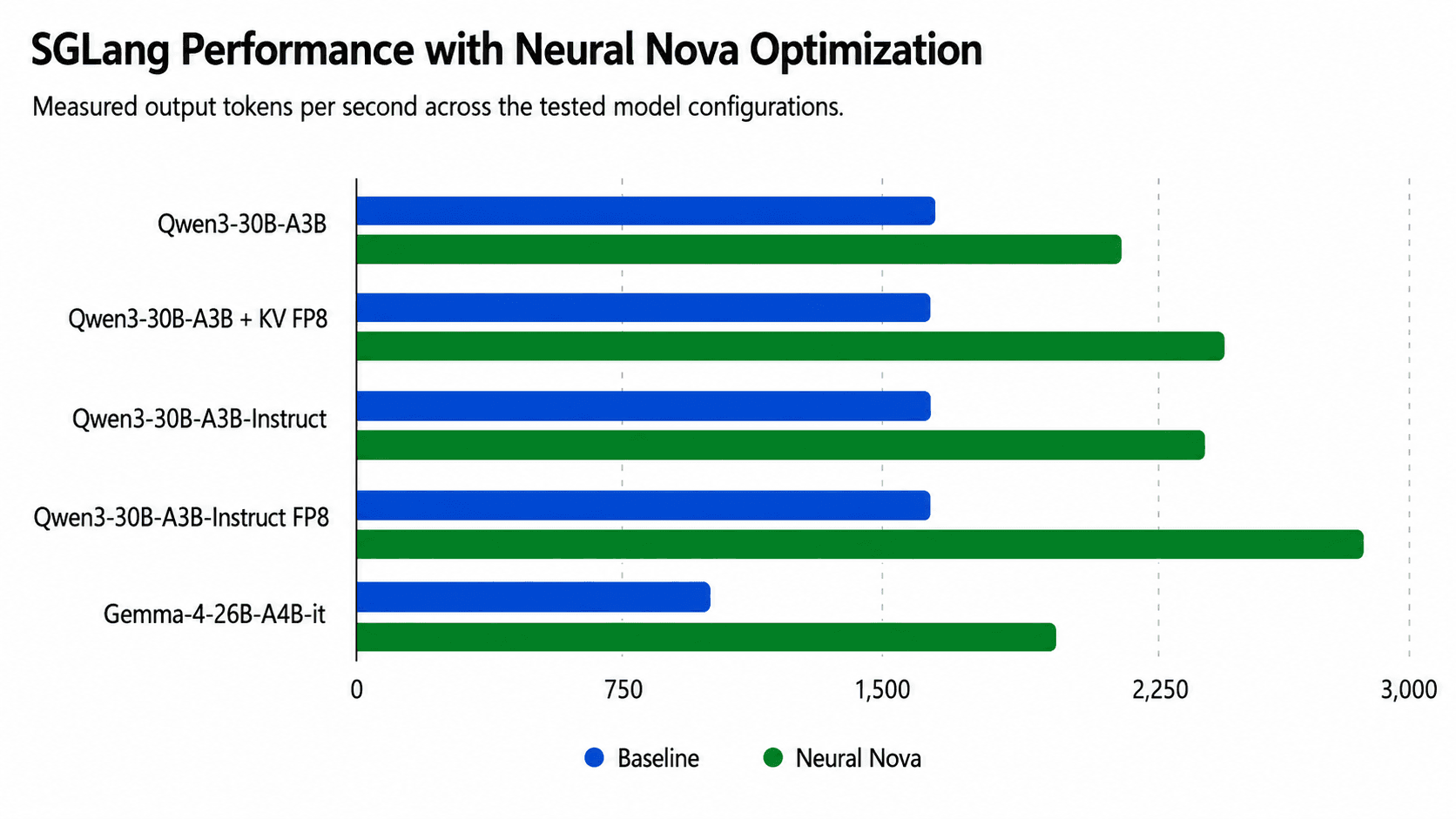
GPU capacity is expensive. For many AI teams, the fastest way to increase serving capacity is not always buying more GPUs — it is improving how the current inference stack schedules, batches, and manages memory. At Neural Nova AI, we recently ran SGLang optimization experiments across several open-weight models, including Qwen3-30B-A3B, Qwen3-30B-A3B-Instruct, and Gemma-4-26B-A4B-it.

The results show that SGLang performance can change significantly when the runtime is tuned for the workload. Without changing the model architecture, retraining the model, or changing the user-facing API, we improved serving throughput by up to 93.7% on the same H100 serving environment.

Across the tested workloads, we observed:

But the more important story is not only the final throughput number. The concurrency sweeps show that the optimized configurations often continue scaling as concurrency increases, while the baseline configurations plateau early. In production, that is what matters: not just whether a server is fast at one benchmark point, but whether it can continue converting higher load into useful throughput before queueing, KV cache pressure, or tail latency becomes unacceptable.

Figure 1: Qwen3-30B SGLang concurrency sweep.

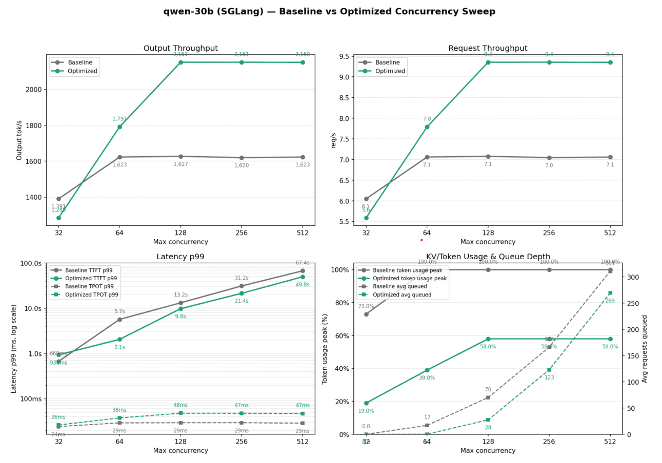
The baseline configuration plateaus around 1,620 output tok/s and 7.1 requests/s, while the optimized configuration scales to approximately 2,150 output tok/s and 9.4 requests/s at higher concurrency.

Figure 2: Qwen3-30B quantized SGLang concurrency sweep.

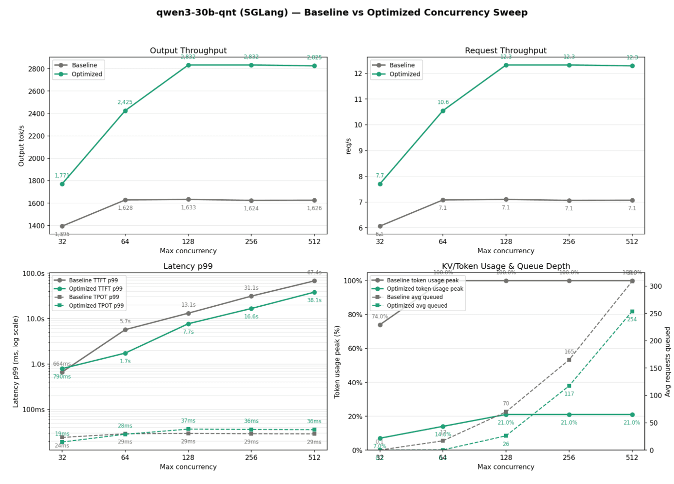
With KV cache quantization, the optimized configuration reaches approximately 2,825–2,833 output tok/s and 12.3 requests/s, while baseline remains near 1,620 output tok/s and 7.1 requests/s.

Figure 3: Qwen3-30B-Instruct SGLang concurrency sweep.

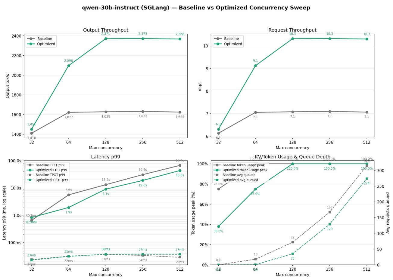
The optimized configuration scales to roughly 2,370 output tok/s and 10.3 requests/s, compared with the baseline plateau near 1,625–1,633 output tok/s and 7.1 requests/s.

Figure 4: Gemma-4-26B SGLang concurrency sweep.

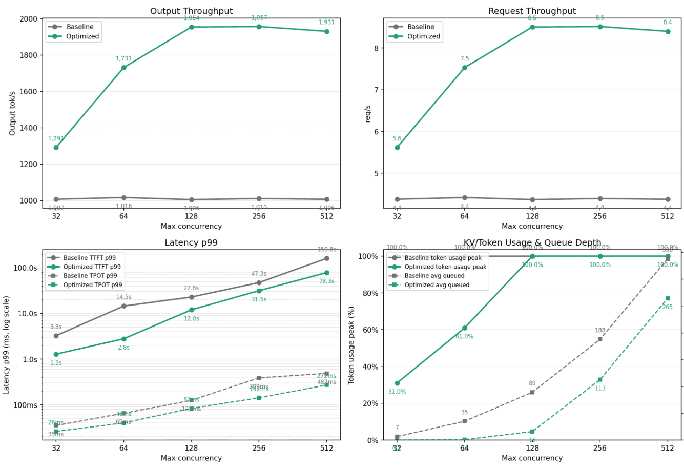
The optimized configuration reaches roughly 1,950 output tok/s and 8.5 requests/s, while baseline remains around 1,010 output tok/s and 4.4 requests/s.

The key lesson is simple:

LLM serving performance is not determined only by the model and the GPU. Runtime configuration can materially change throughput, queue depth, time-to-first-token, tail latency, and GPU efficiency. For inference engineers, this means there is often meaningful performance headroom inside the current serving stack. For VP Engineering and infrastructure leaders, this means optimization can translate directly into more capacity, better user experience, and lower cost per generated token — without immediately expanding the GPU fleet.

Benchmark Environment

These SGLang optimization experiments were run on an NVIDIA H100 CUDA environment using CUDA 12.8. The benchmarks compare baseline and optimized SGLang launch configurations on the same hardware and serving setup. The optimization work focused on runtime-level changes, including KV cache policy, memory allocation, prefill chunking, scheduler behavior, concurrency limits, attention backend selection, and CUDA graph settings.

Because serving performance depends on workload shape, teams should still validate these settings under their own prompt length distribution, output length distribution, request concurrency, latency SLA, and production traffic pattern.

Why We Focused on SGLang

SGLang is an increasingly important serving runtime for high-throughput LLM inference, especially for teams that care about efficient batching, structured generation, memory management, and production observability. But like any inference runtime, the default configuration is general-purpose. Defaults are useful for bringing a server online, but they are rarely optimal for a specific model, traffic shape, latency target, or GPU memory profile.

In production, the best configuration depends on workload-specific factors:

• Prompt length distribution

• Output length distribution

• Request concurrency

• KV cache pressure

• Prefill-to-decode ratio

• GPU memory headroom

• Attention backend behavior

• Latency SLA

• Throughput target

• Queueing behavior under load

Two teams can run the same model on the same hardware and see very different performance depending on how the runtime is configured. That is where execution-layer optimization matters.

Neural Nova AI works below the application layer and above the hardware layer. We optimize serving runtime configuration, scheduling behavior, memory allocation, KV cache policy, quantization strategy, attention backend selection, CUDA graph behavior, and workload-specific benchmarking. The goal is not to make a synthetic benchmark look better. The goal is to improve the real serving behavior that matters in production.

Benchmark Methodology

We compared baseline SGLang launch configurations against optimized configurations across multiple models. The baseline used a standard SGLang server launch with model path, host, port, metrics, and remote-code trust enabled.

The optimized configurations tuned SGLang serving parameters such as:

--mem-fraction-static
--kv-cache-dtype
--chunked-prefill-size
--max-prefill-tokens
--max-running-requests
--schedule-conservativeness
--schedule-policy
--attention-backend
--cuda-graph-max-bs
--enable-mixed-chunk
--stream-interval
--num-continuous-decode-steps

These flags directly affect how SGLang uses GPU memory, how much KV cache capacity is available, how prefill work is chunked, how many requests can run concurrently, and how aggressively the scheduler balances throughput versus latency.

For each run, we evaluated more than a single headline metric. We looked at output throughput, request throughput, end-to-end duration, time-to-first-token, time per output token, inter-token latency, queue depth, running requests, and KV cache utilization. Most importantly, we evaluated performance across a concurrency sweep.

A single benchmark point can be misleading. It may show throughput at one load level, but it does not show where the server saturates. A concurrency sweep reveals whether the system continues scaling as request load increases or whether it plateaus early.

For production inference, this is often the most important question: At what concurrency does my serving stack stop converting more load into more useful throughput?

Concurrency Scaling: Where the Optimization Becomes Visible

The concurrency plots show a consistent pattern across the tested workloads: the baseline configuration reaches its throughput ceiling early, while the optimized configuration often scales to a higher plateau.

This matters because production inference systems are rarely stressed at only one fixed concurrency. Traffic changes throughout the day. User-facing products experience bursts. Model API providers need to handle peak load. Internal AI platforms often serve multiple workloads on shared infrastructure.

In those settings, the question is not only “what is the maximum throughput?” The question is: How much useful throughput can the server maintain as concurrency increases?

Qwen3-30B-A3B

In the Qwen3-30B SGLang sweep, the baseline improves from low concurrency to medium concurrency, then quickly plateaus. Output throughput stays around 1,620–1,627 tok/s from concurrency 64 through 512. Request throughput also remains nearly flat at around 7.0–7.1 req/s.

The optimized configuration behaves differently. At low concurrency, it is slightly slower than baseline. But as max concurrency increases, it continues scaling until it reaches a much higher plateau.

The same pattern appears in request throughput:

This is the production insight: optimization changes the usable concurrency envelope of the server. The baseline reaches saturation early. The optimized setup supports more effective concurrency before flattening.

Qwen3-30B-A3B with KV Quantization

The quantized Qwen3-30B run shows an even stronger scaling pattern.

At concurrency 32, the optimized configuration already outperforms baseline. By concurrency 128, it reaches more than 2,800 output tok/s, while baseline remains around 1,630 output tok/s.

Request throughput follows the same pattern:

This is one of the clearest examples of optimization expanding serving capacity. The optimized system does not merely improve one isolated benchmark point. It shifts the saturation curve upward. KV cache behavior explains part of the gain. In the benchmark summary, KV cache peak dropped from 100% to 14%, and average KV cache usage dropped from 85.6% to 11.1%. Queueing also improved sharply, with average waiting requests dropping from 17.0 to 0.3 in the summarized result. That is why KV cache optimization should not be viewed only as a memory-saving trick. It changes how much concurrent work the server can support before queueing becomes the bottleneck.

Qwen3-30B-A3B-Instruct

The Qwen3-Instruct sweep shows a similar pattern. Baseline throughput plateaus around 1,625–1,633 output tok/s, while the optimized configuration scales to roughly 2,370 output tok/s.

Request throughput also increases from the baseline plateau of around 7.1 req/s to approximately 10.3 req/s under the optimized configuration.

This is relevant for teams serving instruction or reasoning models. These workloads often combine long prompts, variable output lengths, and bursty traffic. Runtime tuning helps the serving stack handle more concurrent demand before hitting its throughput ceiling.

Gemma-4-26B-A4B-it

Gemma-4-26B shows the largest relative improvement. The baseline remains almost flat around 1,000 output tok/s across the concurrency sweep. The optimized configuration scales to approximately 1,950 output tok/s at concurrency 128 and 256.

Request throughput increases from around 4.4 req/s to approximately 8.5 req/s at peak.

This is the most commercially meaningful shape: the baseline is already saturated, while the optimized setup nearly doubles useful serving capacity.

Latency and Queueing Tradeoffs

The concurrency sweeps also show why inference optimization should not be reduced to one metric. As concurrency increases, p99 latency rises in both baseline and optimized configurations. This is expected. Higher concurrency increases pressure on scheduling, memory, queueing, and decode interleaving. The goal is not to make every latency metric improve at every concurrency point. The goal is to find the best operating region for the customer’s workload.

For example, in the non-quantized Qwen3-30B-A3B run, output throughput improves significantly at higher concurrency, but TPOT p99 is higher in the optimized configuration. That means the optimization is moving the system toward higher throughput and better TTFT scaling, but with a decode-latency tradeoff. In contrast, the Qwen3-30B quantized configuration shows a much more balanced improvement. It increases throughput, improves request throughput, reduces KV pressure, and keeps TPOT p99 close to baseline.

This is why production optimization should be tied to the customer’s actual SLA. A customer-facing chatbot may prioritize TTFT and end-to-end p99 latency. A batch summarization workload may prioritize total tokens per second. A model API provider may prioritize request throughput under high concurrency while keeping p99 latency within bounds. An internal platform team may prioritize stable queueing under shared workloads. The optimization strategy should follow the business objective, not the other way around.

Result Highlights

The concurrency sweeps explain how the optimized configurations scale under load. The summarized benchmark results show the net effect on throughput, duration, latency, and KV cache utilization.

Qwen3-30B-A3B with KV Quantization: +49.0% Throughput and Lower Latency

One of the strongest balanced results came from Qwen3-30B-A3B with KV cache quantization. The baseline delivered 1,628 output tok/s. The optimized setup reached 2,425 output tok/s, a 49.0% increase. End-to-end duration dropped from 141.2 seconds to 94.8 seconds, a 32.9% reduction.

Latency improved significantly:

KV cache behavior improved dramatically:

This is the kind of result production teams want: higher throughput, lower latency, lower queueing, and better memory behavior.

Qwen3-30B-A3B-Instruct FP8: +74.1% Throughput

The strongest Qwen3-Instruct result came from the FP8 setup. Output throughput increased from 1,620.8 tok/s to 2,821.8 tok/s, a 74.1% improvement. End-to-end duration dropped from 141.8 seconds to 81.5 seconds, a 42.6% reduction.

This configuration improved every major summarized latency metric:

A 74.1% throughput gain can materially change capacity planning. The same GPU fleet can serve more traffic, absorb higher peak demand, reduce queueing, or lower cost per token.

Gemma-4-26B-A4B-it: +93.7% Throughput

The largest throughput gain came from Gemma-4-26B-A4B-it. The baseline configuration delivered 1,011 output tok/s. The optimized configuration reached 1,957 output tok/s, a 93.7% increase. End-to-end duration dropped from 227.5 seconds to 117.5 seconds, a 48.4% reduction.

Latency improved on several important dimensions:

This result shows that the opportunity is not limited to one model family. Different models respond differently to serving configuration, but the broader pattern is consistent: runtime-level tuning can unlock large gains.

Baseline Cost vs. Optimized GPU Cost

Throughput improvements are not only benchmark wins. They directly affect inference cost. To make the impact concrete, assume an H100 cost of $3.00 per GPU-hour. Actual cost will vary by provider, region, utilization, reserved pricing, and deployment model, but this gives a simple way to estimate the economics.

Cost per 1M output tokens can be estimated as:

Cost per 1M output tokens = GPU hourly cost / output tokens per second × 1,000,000 / 3,600

Using the measured output throughput results:

For example, the Gemma-4-26B-A4B-it result improved output throughput from 1,011 tok/s to 1,957 tok/s. Under the $3.00 per H100-hour assumption, that reduces estimated GPU cost from $0.824 to $0.426 per 1M output tokens, or approximately 48.3% lower GPU cost per generated token.

The Qwen3-30B-A3B-Instruct FP8 result improved throughput from 1,620.8 tok/s to 2,821.8 tok/s. Under the same assumption, estimated GPU cost drops from $0.514 to $0.295 per 1M output tokens, or approximately 42.6% lower cost per generated token.

At fleet scale, the impact becomes more meaningful. For a team spending $100,000 per month on H100 inference capacity for one of these workloads, the equivalent optimized infrastructure cost would be approximately:

The exact dollar savings depend on the customer’s actual H100 cost, utilization rate, traffic pattern, and latency SLA. But the relationship is straightforward: when output tokens per second increase on the same infrastructure, GPU cost per generated token decreases.

What Drove the Gains?

The gains came from tuning multiple parts of the serving stack together. KV cache policy. KV cache capacity often determines how much concurrency a server can support before queueing becomes severe. In the Qwen3 quantized run, KV cache peak dropped from 100% to 14%, and average KV cache usage dropped from 85.6% to 11.1%.

Prefill chunking. Large prompts can monopolize GPU work and delay other requests. Chunked prefill splits prefill into smaller units so SGLang can interleave work more effectively.

Concurrency tuning. Higher concurrency is not always better. If concurrency is too low, the GPU is underutilized. If concurrency is too high, the system may hit memory pressure, queue instability, or worse tail latency.

Scheduler behavior. SGLang scheduling controls can materially affect throughput and queue depth. Parameters such as --schedule-conservativeness and --schedule-policy influence how aggressively the runtime admits and schedules work.

Attention backend selection. Attention backend choice can change performance depending on the model, sequence length, GPU, and serving shape. There is no universal best backend for every workload.

CUDA graph tuning. CUDA graphs can reduce overhead, but the batch size needs to match real serving behavior. Tuning --cuda-graph-max-bs helps align graph capture and replay behavior with the concurrency pattern of the workload.

Why This Matters for AI Infrastructure Teams

Inference optimization directly affects serving economics. If a team can improve throughput by 50%, the same GPU fleet can serve substantially more generated tokens under the tested workload. If a team can improve throughput by 90%, the infrastructure implications are even larger.

This can create several business benefits:

• More traffic served on the same GPUs

• Lower cost per generated token

• Reduced queueing during peak load

• Better user-visible latency

• More headroom for longer context windows

• Delayed GPU expansion

• Higher gross margin for AI products

• Better utilization of expensive accelerator infrastructure

For teams spending heavily on inference, these are not small engineering wins. They affect product scalability, infrastructure budget, and customer experience. This is why inference performance should be treated as a production systems problem, not a one-time benchmark.

How Neural Nova AI Helps

Neural Nova AI helps teams improve AI workload performance on their existing infrastructure. For SGLang, vLLM, and custom inference stacks, we run a technical evaluation to measure the current serving profile, identify bottlenecks, and quantify available performance headroom.

A typical engagement includes:

1. Profiling the current serving setup

2. Measuring throughput, request throughput, TTFT, TPOT, queue depth, and KV cache behavior

3. Running concurrency sweeps to identify the true saturation point

4. Tuning runtime configuration

5. Evaluating KV cache and quantization strategies

6. Testing scheduler and concurrency behavior

7. Comparing attention backend options

8. Validating latency tradeoffs under realistic load

9. Delivering an optimized deployment configuration

The goal is simple: help customers get more performance from the infrastructure they already have. That can mean higher throughput, lower latency, better GPU utilization, or lower cost per token.

Conclusion

Our SGLang optimization results show that significant performance headroom can exist even when the model and hardware stay the same. Across Qwen3-30B-A3B, Qwen3-30B-A3B-Instruct, and Gemma-4-26B-A4B-it, we observed throughput improvements from 32.2% to 93.7%, along with major reductions in TTFT, end-to-end latency, queue depth, and KV cache pressure in several configurations.

The concurrency sweeps reveal the deeper systems story: the optimized configurations often continue scaling to a higher saturation point, while baseline configurations plateau early.

The broader lesson is clear: LLM serving performance is a systems problem.

The model matters. The GPU matters. But so do the serving runtime, scheduler, KV cache policy, memory allocation, attention backend, CUDA graph behavior, and workload-specific concurrency settings. For AI teams scaling inference, optimization should come before overprovisioning.

If your team is running SGLang, vLLM, or a custom LLM serving stack, Neural Nova AI can run a short technical evaluation to measure your current throughput, latency, queueing, concurrency scaling, and KV cache behavior — then identify the optimization headroom before you add more GPUs.