Achieving End-to-End Fine-Tuning Speedup on Qwen-3 automatically with the Nova AI Engine

Neural Nova is an automated kernel optimization system that improves and maintains model performance without changing model architecture, training configuration, or requiring manual kernel tuning. It operates directly on the operator graph, identifying performance-critical operators and generating functionally equivalent, hardware-efficient CUDA kernels. This removes inefficiencies introduced by framework abstractions while preserving numerical correctness and full PyTorch compatibility.

Unlike manual tuning, specialized libraries, or graph-level compilers, Neural Nova targets compute and memory-bound and synchronization-heavy operators that are often left unoptimized. By working at the operator level, it remains architecture-agnostic while capturing low-level performance opportunities beyond compiler reach. Neural Nova targets these gaps directly at the operator execution level.

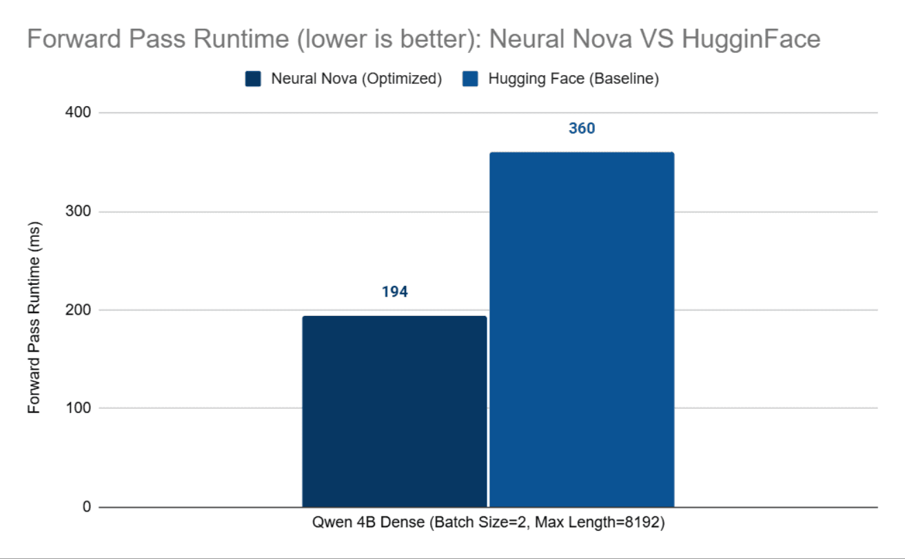
In this post, we demonstrate end-to-end fine-tuning optimization on Qwen-3 (4B and 32B) across single- and multi-GPU setups from a Transformers stack, which we will use as a performance baseline. Model architecture, training logic, and numerical behavior remain unchanged, improving up to 2X for forward pass and 1.11X end-to-end fine-tuning speedup on Qwen-3 with no model or infra changes.

The workflow begins with Nova Parsing, which extracts optimizable operators. Baseline performance is measured at both operator and end-to-end levels, followed by kernel generation, validation, and full pipeline integration.

In the Qwen-3 model, execution we primarily focus on RMSNorm.

Each identified operator is passed to the Neural Nova AI Engine, which generates CUDA kernel implementations while applying internally developed optimization techniques. All generated kernels undergo validations mentioned before being composed back into the optimized model.

We begin with RMSNorm, which normalizes hidden states by scaling each element with the reciprocal square root of the mean squared activations, followed by a per-channel weight multiplication. It is described as follows:

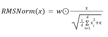
Where: 

• x= (x1, ... , xd): input hidden state

• d: hidden dimension

• ϵ : small constant for numerical stability

• w E Rd: learnable per-channel (per-feature) weight

• ⊙: element-wise multiplication

Below is the reference PyTorch implementation of RMSNorm used in the Qwen-3 model.

Pytorch Operators

@use_kernel_forward_from_hub("RMSNorm")
class Qwen3RMSNorm(nn.Module):
    def __init__(self, hidden_size, eps: float = 1e-6) -> None:
        """
        Qwen3RMSNorm is equivalent to T5LayerNorm
        """
        super().__init__()
        self.weight = nn.Parameter(torch.ones(hidden_size))
        self.variance_epsilon = eps

    def forward(self, hidden_states: torch.Tensor) -> torch.Tensor:
        input_dtype = hidden_states.dtype
        hidden_states = hidden_states.to(torch.float32)
        variance = hidden_states.pow(2).mean(-1, keepdim=True)
        hidden_states = hidden_states * torch.rsqrt(variance + self.variance_epsilon)
        return self.weight * hidden_states.to(input_dtype)

Optimization Strategy

The optimized RMSNorm kernel applies the following techniques:

• Thread-block–strided reduction: Instead of assigning a single element per thread, elements are processed using a block-level stride, enabling parallel accumulation of squared values across threads within a block.
  
  

• Shared-memory reduction: Intermediate reduction results are stored in shared memory, reducing global memory traffic and improving utilization of the GPU memory hierarchy.
  
  

• Coalesced memory access: The access pattern
  for (int i = tid; i < hidden_size; i += BlockSize)
ensures that threads within a warp access contiguous memory locations, resulting in coalesced global memory accesses for typical hidden sizes.
  
  

• Operator fusion: Variance computation, normalization, and weight scaling are fused into a single kernel launch, eliminating intermediate tensors and reducing kernel launch overhead.
  
  

• Block-level reuse of normalization factor: The normalization factor is computed once per row and stored in shared memory, allowing all threads within the block to reuse it without redundant computation.

Accumulation is performed in FP32 to preserve numerical stability, while synchronization is limited to the minimum required for correctness.

Optimized CUDA Kernels Snippet    

  // Step 1: Compute sum of squares for the row in float32
    float sum_sq = 0.0f;
    for (int i = tid; i < hidden_size; i += BlockSize) {
        scalar_t val = input[row * hidden_size + i];
        float val_f = static_cast<float>(val);
        sum_sq += val_f * val_f;
    }
    // Shared memory for block-wide reduction
    __shared__ float s_sum[BlockSize];
    s_sum[tid] = sum_sq;
    __syncthreads();
    // Parallel reduction in shared memory
    for (int stride = BlockSize / 2; stride > 0; stride >>= 1) {
        if (tid < stride) {
            s_sum[tid] += s_sum[tid + stride];
        }
        __syncthreads();
    }
    // Compute normalization factor and broadcast to all threads
    if (tid == 0) {
        float mean_sq = s_sum[0] / static_cast<float>(hidden_size);
        s_sum[0] = rsqrtf(mean_sq + epsilon);
    }
    __syncthreads();
    float norm_factor = s_sum[0];
    // Step 2: Normalize and apply weight
    for (int i = tid; i < hidden_size; i += BlockSize) {
        scalar_t val = input[row * hidden_size + i];
        float val_f = static_cast<float>(val);
        float normalized = val_f * norm_factor;
        output[row * hidden_size + i] = static_cast<scalar_t>(normalized) * weight[i];
    }
}

We then validated functional correctness by generating random input tensors and comparing the outputs of the optimized kernels against the corresponding PyTorch operators. Since all operators produce float32 outputs, we used PyTorch’s standard relative (rtol) and absolute (atol) tolerances to account for minor numerical differences.

In addition, we benchmarked execution time in milliseconds (ms) and power draw (watts) against both PyTorch native execution and torch.compile. For each configuration, benchmarks were run for 1,000 iterations to minimize system noise and obtain stable, reliable performance measurements. We conducted testing and benchmark on the NVIDIA H100 GPU. Below are our results:

RmsNorm

{

    "max_diff": 4.768e-07,

    "cuda_runtime": 0.029,

    "torch_runtime": 0.149,

    "torch_compile_runtime": 0.249,

    "speedup_over_pytorch": 5.026,

    "speedup_over_torch_compile": 8.362,

    "dimension_match": true,

    "cuda_power": 122.337,

    "torch_power": 122.526,

    "torch_compile_power": 125.372,

    "correct": true

}

RMSNorm achieves 5× speedup over PyTorch and 8× over torch.compile. The optimized kernel significantly outperforms the PyTorch operator in both native and torch.compile modes while maintaining identical power draw. The speedup comes from eliminating framework overhead, enforcing contiguous memory access, and executing the entire operation in a single, specialized kernel with minimal dispatch and control logic. 

In contrast, torch.compile can be slower than native PyTorch for small or already-optimized, memory-bound kernels, where compilation overhead and limited fusion opportunities outweigh its benefits. Its strength is on large graph fusion, not microkernels. 

As we previously showed significant improvements of our Forward Pass on the real fine-tuning case from the previous blog "Why Custom CUDA Kernels via PyBind11 Can Outperform Pure PyTorch in LLM Fine-Tuning", we will move onto the second key component of the LLM, Backward Pass.

Backward Pass Kernel

We implement a custom backward pass, ensuring the model can properly perform both forward and backward computations during fine-tuning.

Our optimized RMSNorm backward kernel uses a two-pass design. In the first pass, each block computes the row-wise statistics needed for backward propagation, including the sum of squared activations and the gradient-weighted dot product. These reductions are performed at the block level and shared across threads through shared memory. In the second pass, the kernel computes both grad_input and grad_weight directly.

Several optimizations are applied: block-level parallel reduction, shared-memory reuse of common normalization terms, FP32 accumulation for numerical stability, thread-block–strided access for parallelism, and fused gradient computation within a single kernel launch. The kernel also uses atomicAdd for grad_weight, avoiding an additional global workspace or separate reduction kernel. This design reduces launch overhead, improves memory efficiency, and keeps the backward computation compact and hardware-aware.

template <typename scalar_t, int BlockSize>
__global__ void rmsnorm_backward_kernel(
    const scalar_t* __restrict__ grad_output,
    const scalar_t* __restrict__ input,
    const scalar_t* __restrict__ weight,
    scalar_t* __restrict__ grad_input,
    float* __restrict__ grad_weight,
    int hidden_size,
    float epsilon) 
{
    int row = blockIdx.x;
    int tid = threadIdx.x;

    float sum_sq = 0.0f;
    float dot_prod = 0.0f;

    // First Pass: Calculate shared statistics
    for (int i = tid; i < hidden_size; i += BlockSize) {
        float x = static_cast<float>(input[row * hidden_size + i]);
        float gy = static_cast<float>(grad_output[row * hidden_size + i]);
        float w = static_cast<float>(weight[i]);

        sum_sq += x * x;
        dot_prod += gy * w * x;
    }

    float m_sum_sq = blockReduceSum<float, BlockSize>(sum_sq);
    float m_dot_prod = blockReduceSum<float, BlockSize>(dot_prod);

    __shared__ float common_rsqrt;
    __shared__ float common_c;

    if (tid == 0) {
        float r = rsqrtf(m_sum_sq / hidden_size + epsilon);
        common_rsqrt = r;
        common_c = (m_dot_prod * r * r) / hidden_size;
    }
    __syncthreads();

    float r_val = common_rsqrt;
    float c_val = common_c;

    // Second Pass: Compute gradients
    for (int i = tid; i < hidden_size; i += BlockSize) {
        float x = static_cast<float>(input[row * hidden_size + i]);
        float gy = static_cast<float>(grad_output[row * hidden_size + i]);
        float w = static_cast<float>(weight[i]);

        // grad_input calculation
        float gi = r_val * (gy * w - x * c_val);
        grad_input[row * hidden_size + i] = static_cast<scalar_t>(gi);

        // grad_weight calculation - Use atomicAdd to avoid global workspace and second kernel
        float gw = gy * (x * r_val);
        atomicAdd(&grad_weight[i], gw);
    }
}

We tested the correctness of our optimized backward pass against the baseline by calculating the grad inputs and the MSE and Cosine similarity between their grad weights using double data type that ensures full accuracy. All metrics demonstrate that the accuracy between optimized and baseline backward passes are identical. After testing is sucesssful, the data type will be converted back to data types from baseline, which is BF16, to ensure that the fine-tuning accuracy maintains identical precision.

We also tested the backward pass speedups between them to determine if our optimized backward pass is faster. Our result shows that our optimized backward pass achieves 5% speedups compared to the baseline:

Kernel Integration

After optimizing the kernels, we integrated them back into the PyTorch model as custom operators using Pybind11 and Python bindings. First, we instantiate the C++ kernel interface for each kernel and bind them using Pybind11 as shown:

PYBIND11_MODULE(TORCH_EXTENSION_NAME, m) {
    m.def("forward", &forward, "RMSNorm forward");
    m.def("backward", &backward, "RMSNorm backward");
}

Next, we put our Python interface of optimized Forward and backward passes on the model class here:

class Qwen3RMSNormFunction(torch.autograd.Function):
    @staticmethod
    def forward(ctx, hidden_states, weight, variance_epsilon):
        ctx.save_for_backward(hidden_states, weight)
        ctx.variance_epsilon = variance_epsilon
        return neuralnova_qwen3_rms_norm.forward(hidden_states, weight, variance_epsilon)

    @staticmethod
    def backward(ctx, grad_output):
        if _rmsnorm_backward is None:
            raise NotImplementedError("neuralnova_qwen3_rms_norm._C.backward is not available.")
        hidden_states, weight = ctx.saved_tensors
        grad_input, grad_weight = _rmsnorm_backward(
            grad_output,
            hidden_states,
            weight,
            ctx.variance_epsilon
        )
        return grad_input, grad_weight, None

We integrate our optimization changes as an enhanced Transformers framework so we will fine-tune our stack version against the Vanilla Transformers stack.

After validating functional correctness and benchmarking all optimized kernels, we fine-tune both the baseline and optimized QWEN3 models on real-world data from Nemotron-Post-Training-Dataset-v2, focusing on mathematics and programming tasks. During training, we measure tokens per second at each iteration to capture end-to-end speedups, including forward, backward, and optimizer steps. After fine-tuning, we evaluate both model variants on standard benchmarks—HumanEval, Competition Math, LiveCodeBench, and AIME 2025—to compare accuracy. Below, we report the configurations and  performance results of the optimized model versus the baseline.

Configurations : 
Model: Qwen/Qwen3-4B-Instruct-2507
Dataset: nvidia/Nemotron-Post-Training-Dataset-v2 (split: math,code)
Max Train Samples: 1000
Batch Size: 2 (per device)
Gradient Accumulation: 2
Epochs: 1 
Max Length: 8192
Learning Rate: 2e-5
Precision: bfloat16
Hardware: NVIDIA H100 GPU
Software :
CUDA : 13.0
Pytorch : 2.10
Transformers : 4.57

Results : 

Baseline: 6,000 Tokens/seconds 

Optimized Version: 6,700 Tokens/seconds

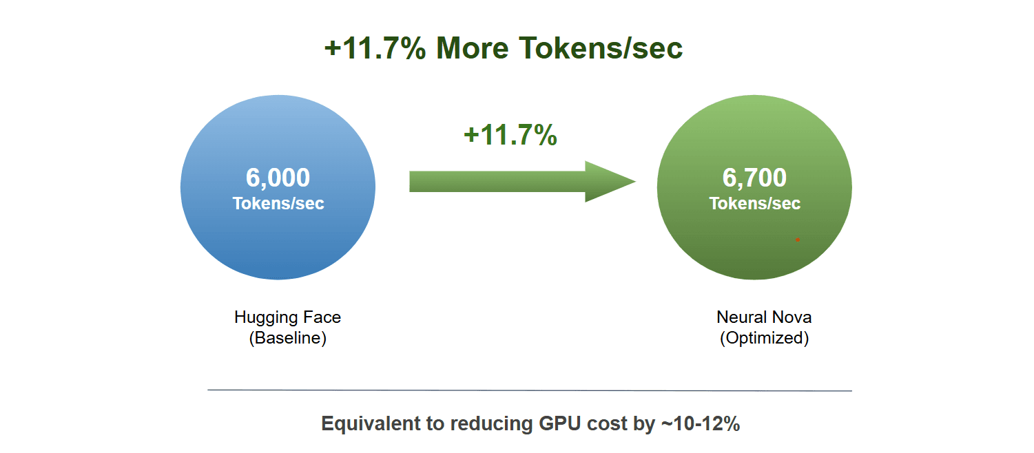
The optimized Qwen3 model delivers an 11% throughput improvement over the baseline, achieved automatically by the Nova AI Engine with no manual effort, while preserving evaluation accuracy across all benchmarks. This also translates to ~11% reduction in GPU hours, improving cost efficiency for large-scale training workloads. These results demonstrate that kernel-level optimizations can drive meaningful end-to-end performance gains in real-world settings.

We further extend this approach to larger models, scaling optimized forward and backward kernels to 32B parameter models using multi-GPU setups and LoRA. This shows that Nova’s optimizations generalize across both small and large models, and support single- and multi-GPU environments. The optimization generalizes to 32B models on 8×H100, achieving consistent throughput gains in multi-GPU settings.

Configurations : 
Model: Qwen/Qwen3-32B
Dataset: nvidia/Nemotron-Post-Training-Dataset-v2 (split: math,code)
Max Train Samples: 1000
Batch Size: 1 (per device)
Epochs: 1 
lora_r: 8
lora_alpha: 16 
Gradient Accumulation: 2
Max Length: 4096
use_lora: true
Learning Rate: 2e-5
Precision: bfloat16
Hardware: 8 NVIDIA H100 GPUs
Software :
CUDA : 13.0
Pytorch : 2.10
Transformers : 4.57

Results : 

Baseline: 6,751 Tokens/seconds 

Optimized Version: 7,505 Tokens/seconds

Fine-Tuning Accuracy test

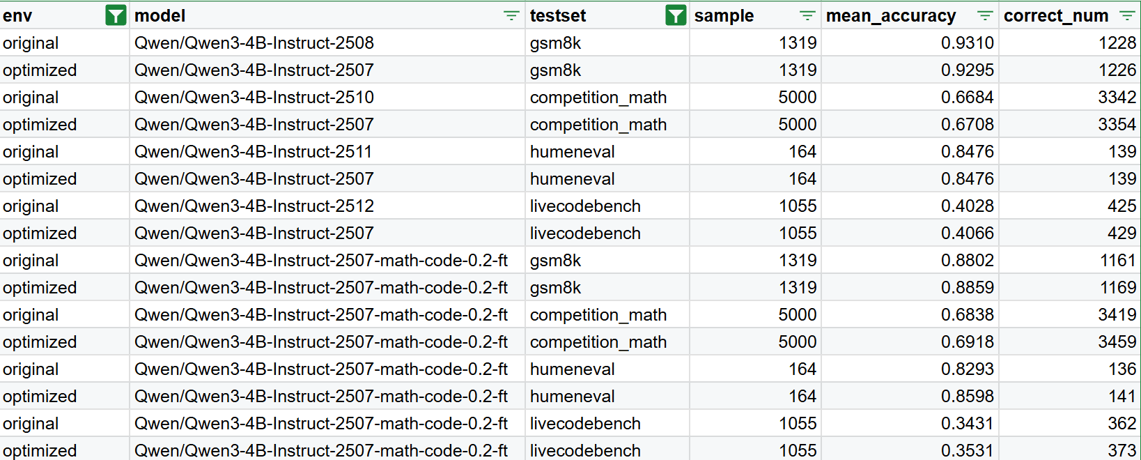
Next, we evaluate the accuracy of the Qwen3 models on mathematics and programming tasks for both the baseline and optimized versions. We report results before and after fine-tuning (0.2-ft) to assess stability and performance changes. The optimized model achieves accuracy comparable to the baseline across all evaluations, indicating that the kernel optimizations preserve functional correctness while delivering performance improvements.

Conclusion

We demonstrate that meaningful performance gains still remain beyond today’s compiler and inference stacks. Without modifying model architecture, infrastructure, or batch size, we achieve an 11% end-to-end reduction in training cost on Qwen-3 and scale our optimization from single to multi-GPU cases on NVIDIA H100 GPU—purely by optimizing execution at the operator level. This highlights that operator-level optimization can unlock real-world training speedups beyond the reach of graph-level compilers for memory and synchronization-bound workloads.

By automatically identifying performance-critical operators and generating hardware-efficient CUDA kernels, Neural Nova outperforms both native PyTorch and torch.compile, while preserving numerical correctness and maintaining identical power draw, translating directly into higher effective GPU utilization and lower cost per token when integrated into a full Transformers pipeline.

This represents one layer of optimization, with further opportunities ahead. Additional improvements can be achieved through techniques such as KV caching, quantization, and sparsity, which we plan to explore in future work. Additionally, Neural Nova does not stop at initial optimization—we also continuously maintains performance across CUDA, driver, and hardware changes on real production workloads.